This walkthrough is also available as a Jupyter ipynb Notebook - you can run yourself
Half of the fun with Jupyter Notebooks is organizing the data how you want.
But the most important part is how you can tell a story with that data.
The jupyter-ijavascript-utils library tries to give you a few different options:
Showing your data through a Table
utils = require('jupyter-ijavascript-utils');
['utils'];
[ 'utils' ]
JSON.stringify(
    utils.datasets.list().slice(0, 10)
);
'["annual-precip.json","anscombe.json","barley.json","budget.json","budgets.json","burtin.json","cars.json","countries.json","crimea.json","driving.json"]'
utils.ijs.await(async($$, console) => {
    cars = await utils.datasets.fetch('cars.json');
    console.log(`You have loaded ${cars.length} number of cars`);
});
You have loaded 406 number of cars
For more on tables, see the Exporting and Tables tutorial
utils.table(cars)
    .limit(10)
    .filter((car) => car.Name.startsWith('chevrolet'))
    .sort('-Name')
    .styleRow(({record}) => record.Miles_per_Gallon > 20
             ? 'background-color:lightcyan' : '')
    .render(10);
| Name | Miles_per_Gallon | Cylinders | Displacement | Horsepower | Weight_in_lbs | Acceleration | Year | Origin |
|---|---|---|---|---|---|---|---|---|
| chevrolet woody | 24.5 | 4 | 98 | 60 | 2,164 | 22.1 | 1976-01-01 | USA |
| chevrolet vega 2300 | 28 | 4 | 140 | 90 | 2,264 | 15.5 | 1971-01-01 | USA |
| chevrolet vega (sw) | 22 | 4 | 140 | 72 | 2,408 | 19 | 1971-01-01 | USA |
| chevrolet vega | 20 | 4 | 140 | 90 | 2,408 | 19.5 | 1972-01-01 | USA |
| chevrolet vega | 21 | 4 | 140 | 72 | 2,401 | 19.5 | 1973-01-01 | USA |
| chevrolet vega | 25 | 4 | 140 | 75 | 2,542 | 17 | 1974-01-01 | USA |
| chevrolet nova custom | 16 | 6 | 250 | 100 | 3,278 | 18 | 1973-01-01 | USA |
| chevrolet nova | 15 | 6 | 250 | 100 | 3,336 | 17 | 1974-01-01 | USA |
| chevrolet nova | 18 | 6 | 250 | 105 | 3,459 | 16 | 1975-01-01 | USA |
| chevrolet nova | 22 | 6 | 250 | 105 | 3,353 | 14.5 | 1976-01-01 | USA |
Showing Through Vega Charts
For more, see the Vega Charting Tutorial
Vega-Lite
Vega-Lite is a charting library that provides a great deal of flexibility and interaction
while also allowing for very simple use cases
(and further simplified with Vega-Lite-Api)
More examples and detail can be found on the Vega module
Vega
It is built on Vega that uses d3 as a visualization kernel.
True Vega is also supported, providing support for additional capabilities (that to my knowledge cannot be done with vega-lite)
- such as Radar Charts,
- Contour Plots,
- Tree Layouts,
- Force Plots,
- and others.
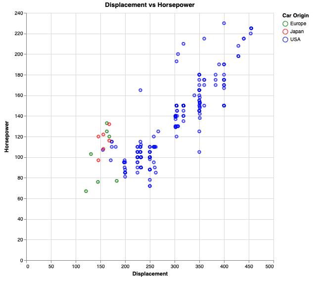
utils.vega.svg((vl) => vl.markPoint()
  .data(cars)
  .title('Displacement vs Horsepower')
  .width(500)
  .height(500)
  .transform(
    vl.filter('datum.Cylinders > 4')
  )
  .encode(
    //-- Qualitiative field - a number
    //-- that can have the position determined relative to another and charted
    vl.x().fieldQ('Displacement'),
    vl.y().fieldQ('Horsepower'),
    vl.color().fieldN('Origin').title('Car Origin').scale({ range: ['green', 'red', 'blue'] })
  )
)
Data Driven Maps

Interactive Charts
Rendering Maps
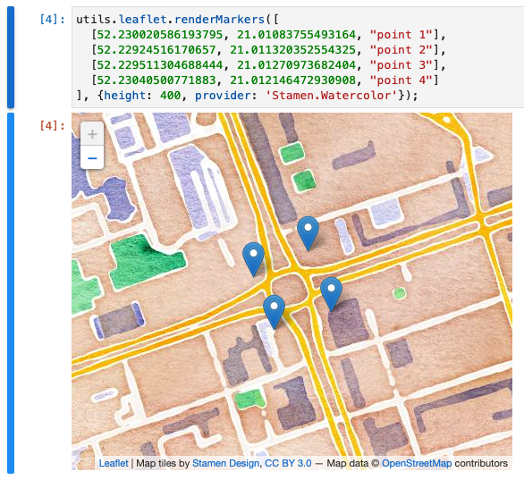
You can use the Leaflet module to render maps, or markers.
This leverages Leaflet and Leaflet-Provider to help you show locations, geometries, etc.
Please see the leaflet module for more
utils.leaflet.renderMarkers([
  [52.230020586193795, 21.01083755493164, "point 1"],
  [52.22924516170657, 21.011320352554325, "point 2"],
  [52.229511304688444, 21.01270973682404, "point 3"],
  [52.23040500771883, 21.012146472930908, "point 4"]
], {height: 400, provider: 'Stamen.Watercolor'});
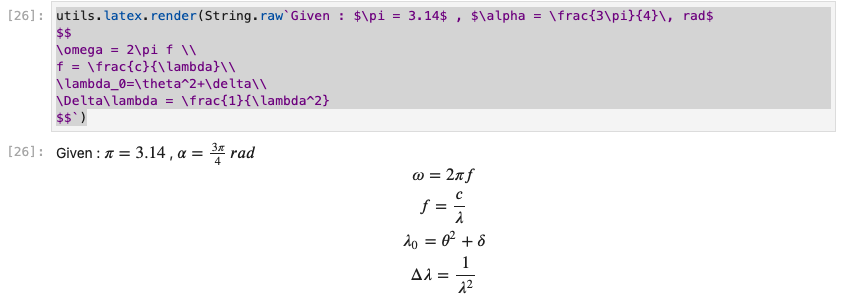
Render Equations using Latex
Both LaTeX and KaTeX are supported.
LaTeX is a typesetting engine often used for writing mathematical formulas along with technical and scientific documentation.
KaTeX is a very fast typesetting library specifically to write math notation. It implements a subset of the LaTeX specification.
Please see the latex module for more
utils.latex.render(String.raw`Given : $\pi = 3.14$ , $\alpha = \frac{3\pi}{4}\, rad$
$$
\omega = 2\pi f \\
f = \frac{c}{\lambda}\\
\lambda_0=\theta^2+\delta\\
\Delta\lambda = \frac{1}{\lambda^2}
$$`);
Given : $\pi = 3.14$ , $\alpha = \frac{3\pi}{4}, rad$ $$ \omega = 2\pi f \ f = \frac{c}{\lambda}\ \lambda_0=\theta^2+\delta\ \Delta\lambda = \frac{1}{\lambda^2} $$
Render Diagrams through PlantUML
PlantUML Render diagrams in Jupyter Lab Renderer for PlantUML - a rendering engine that converts text to diagrams.
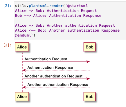
All PlantUML diagrams are supported - as they are managed by the server.
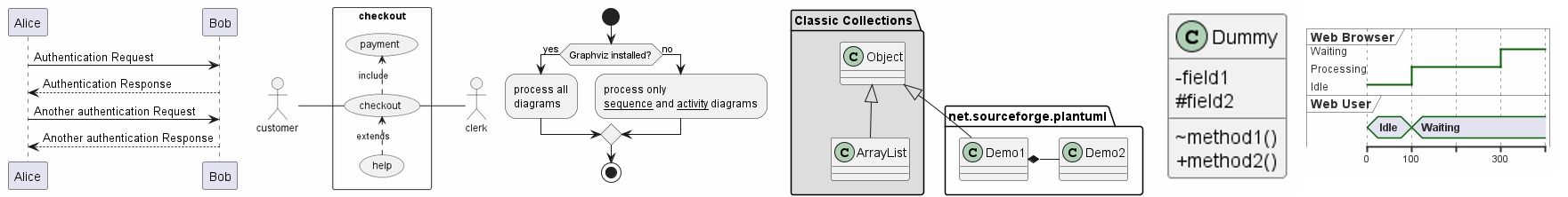
Such as:
- Sequence diagrams,
- Usecase diagrams,
- Class diagrams,
- Object diagrams,
- Activity diagrams,
- Component diagrams,
- Deployment diagrams,
- State diagrams,
- Timing diagrams,
- and many others...
Please see the PlantUML module for more
Dynamically Generate SVGs for Diagrams
The utility here is a wrapper for SVG.js, so SVGs can be rendered either Server-Side (within the Notebook) or Client Side (within the browser rendering the notebook - but lost on export)
  utils.svg.render({ width: 400, height: 200,
      onReady: ({el, width, height, SVG }) => {
          const yellowTransition = new SVG.Color('#FF0000').to('#00FF00');
          for (let i = 0; i <=5; i++){
              el.rect(100, 100)
                  .fill(yellowTransition.at(i * 0.2).toHex())
                  .transform(
                      new SVG.Matrix()
                          .translate(i * 20, 0)
                          .rotate(45)
                          .translate(100, 0)
                  );
          }
      }
  })

This also can be rendered on the client side to create your own animations.
utils.svg.embed(({ el, SVG, width, height }) => {
    var rect1 = el.rect(100, 100)
        .move(width/2, 0);

    rect1.animate(1000, 0, 'absolute')
        .move(width/2, 100)
        .loop(true, true);
})

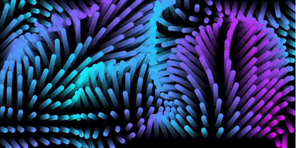
Leveraging Noise you can make some very interesting images even without data.
Extending with HTML Script
By balancing computing between the client and the browser side (through HTMLScript) you can leverage additional libraries that can use the DOM.
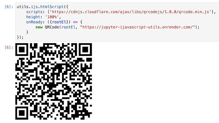
For more, please see the Architecture section and the HTMLScript tutorial